正文
43 - What is machine learning anyway
- Machine Learning 机器学习
- Supervised Learning 监督学习
- Classification problem 分类问题
- Support Vector Machines 支持向量机
- Discriminant Analysis 判别分析法
- Naive Bayes 朴素贝叶斯
- Nearest Neighbor 邻近算法
- Regression 回归
- Linear Regression, GLM 线性回归,广义线性模型
- SVR, GPR 支持向量回归,高斯过程回归
- Ensemble Methods 集成学习算法
- Decision Trees 决策树
- Neural Networks 神经网络
- Classification problem 分类问题
- Unsupervised Learning 无监督学习
- Clustering 聚类
- K-Means, K-Medoids, Fuzzy C-Means
- Hierarchical 层次聚类
- Gaussian Mixture 高斯混合模型
- Neural Networks 神经网络
- Hidden Markov Model 隐马尔科夫模型
- Clustering 聚类
- Supervised Learning 监督学习
- Machine Learning VS Deep Learning
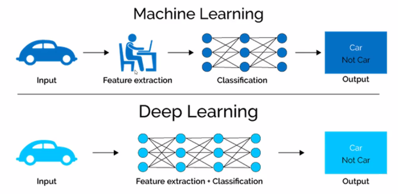
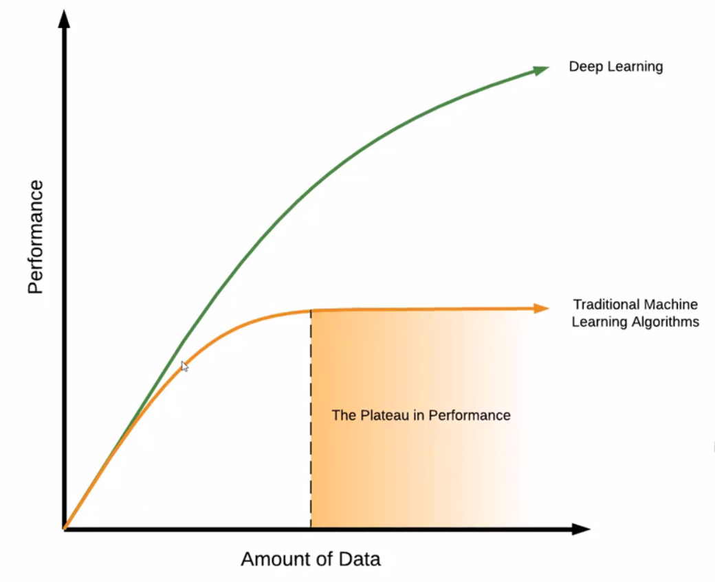
在数据量大的情况下使用深度学习效果更好。
44 - What is linear regression
介绍了下线性回归以及损失函数。
45 - Linear regression using Sci-Kit Learn in Python
python
import pandas as pd
import numpy as np
import matplotlib.pyplot as plt
from sklearn import linear_model

df = pd.read_csv('data/cells.csv')
df| time | cells | |
|---|---|---|
| 0 | 0.0 | 205 |
| 1 | 0.5 | 225 |
| 2 | 1.0 | 238 |
| 3 | 1.5 | 240 |
| 4 | 2.0 | 248 |
| 5 | 2.5 | 260 |
| 6 | 3.0 | 265 |
| 7 | 3.5 | 283 |
| 8 | 4.0 | 301 |
| 9 | 4.5 | 305 |
| 10 | 5.0 | 309 |
python
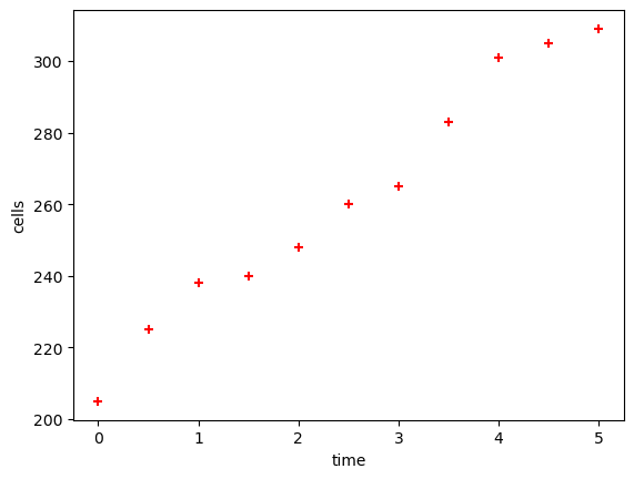
plt.xlabel('time')
plt.ylabel('cells')
plt.scatter(df.time, df.cells, color='red', marker='+')
<matplotlib.collections.PathCollection at 0x2c7bd4eb0d0>
-
x independent (time)
-
y dependent - we are predicting Y
python
x_df = df[['time']]
x_df| time | |
|---|---|
| 0 | 0.0 |
| 1 | 0.5 |
| 2 | 1.0 |
| 3 | 1.5 |
| 4 | 2.0 |
| 5 | 2.5 |
| 6 | 3.0 |
| 7 | 3.5 |
| 8 | 4.0 |
| 9 | 4.5 |
| 10 | 5.0 |
python
x_df.dtypestime float64
dtype: object
python
y_df = df.cells- 创建并训练模型
python
reg = linear_model.LinearRegression()  # Create an instance of the model
reg.fit(x_df, y_df) # Training the model (fitting a line)- 预测模型
python
# Predict
reg.predict([[2.3]])
C:\Users\gzjzx\anaconda3\lib\site-packages\sklearn\base.py:450: UserWarning: X does not have valid feature names, but LinearRegression was fitted with feature names
warnings.warn(
array([257.61090909])
- 评分
python
reg.score(x_df, y_df)0.9784252641866715
- Y = mx + C
python
c = reg.intercept_
m = reg.coef_
2.3 * m + c
array([257.61090909])
- 预测多个数据
python
cells_predict_df = pd.read_csv('data/cells_predict.csv')
cells_predict_df.head()| time | |
|---|---|
| 0 | 0.1 |
| 1 | 0.2 |
| 2 | 0.3 |
| 3 | 0.4 |
| 4 | 0.5 |
python
predicted_cells = reg.predict(cells_predict_df)
predicted_cells
array([212.33090909, 214.38909091, 216.44727273, 218.50545455,
220.56363636, 222.62181818, 224.68 , 226.73818182,
228.79636364, 230.85454545, 232.91272727, 234.97090909,
237.02909091, 239.08727273, 241.14545455, 243.20363636,
245.26181818, 247.32 , 249.37818182, 251.43636364,
253.49454545, 255.55272727, 257.61090909, 259.66909091,
261.72727273, 263.78545455, 265.84363636, 267.90181818,
269.96 , 272.01818182, 274.07636364, 276.13454545,
278.19272727, 280.25090909, 282.30909091, 284.36727273,
286.42545455, 288.48363636, 290.54181818, 292.6 ])
- 将预测数据合并并保存
python
cells_predict_df['cells'] = predicted_cells
cells_predict_df.head()| time | cells | |
|---|---|---|
| 0 | 0.1 | 212.330909 |
| 1 | 0.2 | 214.389091 |
| 2 | 0.3 | 216.447273 |
| 3 | 0.4 | 218.505455 |
| 4 | 0.5 | 220.563636 |
python
cells_predict_df.to_csv('predicted_cells.csv')46 - Splitting data into training and testing sets for machine learning
python
import pandas as pd
import numpy as np
import matplotlib.pyplot as plt
from sklearn import linear_model
python
df = pd.read_csv('data/cells.csv')
df| time | cells | |
|---|---|---|
| 0 | 0.0 | 205 |
| 1 | 0.5 | 225 |
| 2 | 1.0 | 238 |
| 3 | 1.5 | 240 |
| 4 | 2.0 | 248 |
| 5 | 2.5 | 260 |
| 6 | 3.0 | 265 |
| 7 | 3.5 | 283 |
| 8 | 4.0 | 301 |
| 9 | 4.5 | 305 |
| 10 | 5.0 | 309 |
python
x_df = df.drop('cells', axis='columns')
y_df = df.cells- 分割训练集(train)和测试集(test)
python
from sklearn.model_selection import train_test_split

X_train, X_test, y_train, y_test = train_test_split(x_df, y_df, test_size=0.4, random_state=10)
python
X_train| time | |
|---|---|
| 10 | 5.0 |
| 3 | 1.5 |
| 1 | 0.5 |
| 0 | 0.0 |
| 4 | 2.0 |
| 9 | 4.5 |
python
reg = linear_model.LinearRegression()
reg.fit(X_train, y_train)

prediction_test = reg.predict(X_test)
prediction_test
array([229.66081871, 270.73684211, 291.2748538 , 260.46783626,
281.00584795])
- 计算均方误差
python
print('Mean sq. error between y_test and predicted =', np.mean(prediction_test - y_test) ** 2)Mean sq. error between y_test and predicted = 7.677112273861912
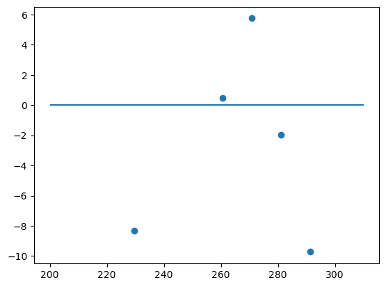
- 计算残差
python
plt.scatter(prediction_test, prediction_test - y_test)
plt.hlines(y=0, xmin=200, xmax=310)  # 画一条水平线
<matplotlib.collections.LineCollection at 0x26a2470d640>
47 - Multiple Linear Regression with SciKit-Learn in Python
python
import pandas as pd

df = pd.read_excel('data/images_analyzed.xlsx')
df.head()| User | Time | Coffee | Age | Images_Analyzed | |
|---|---|---|---|---|---|
| 0 | 1 | 8 | 0 | 23 | 20 |
| 1 | 1 | 13 | 0 | 23 | 14 |
| 2 | 1 | 17 | 0 | 23 | 18 |
| 3 | 1 | 22 | 0 | 23 | 15 |
| 4 | 1 | 8 | 2 | 23 | 22 |
python
import seaborn as sns

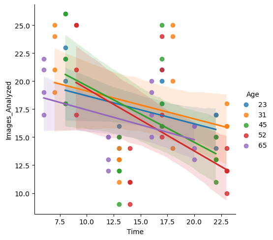
sns.lmplot(x='Time', y='Images_Analyzed', data=df, hue='Age')
<seaborn.axisgrid.FacetGrid at 0x238adc47910>
python
import numpy as np
from sklearn import linear_model

reg = linear_model.LinearRegression()
reg.fit(df[['Time', 'Coffee', 'Age']], df.Images_Analyzed)

reg.coef_, reg.intercept_
(array([-0.35642282, -0.3475 , -0.04279945]), 25.189636192124166)
python
reg.predict([[13, 2, 23]])C:\Users\gzjzx\anaconda3\lib\site-packages\sklearn\base.py:450: UserWarning: X does not have valid feature names, but LinearRegression was fitted with feature names
warnings.warn(
array([18.8767522])
48 - What is logistic regression
虽然是 Regression,不过主要用于 Classfication (二分类问题)。
逻辑回归(Logistic Regression)(一) - 知乎 (zhihu.com)
49 - Logistic Regression using scikit-learn in Python
- STEP1: DATA READING AND UNDERSTANDING
python
import pandas as pd
from matplotlib import pyplot as plt

df = pd.read_csv('data/images_analyzed_productivity1.csv')
df.head()| User | Time | Coffee | Age | Images_Analyzed | Productivity | |
|---|---|---|---|---|---|---|
| 0 | 1 | 8 | 0 | 23 | 20 | Good |
| 1 | 1 | 13 | 0 | 23 | 14 | Bad |
| 2 | 1 | 17 | 0 | 23 | 18 | Good |
| 3 | 1 | 22 | 0 | 23 | 15 | Bad |
| 4 | 1 | 8 | 2 | 23 | 22 | Good |
python
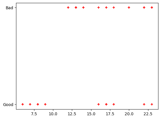
plt.scatter(df.Time, df.Productivity, marker='+', color='red')<matplotlib.collections.PathCollection at 0x206c9140bb0>
python
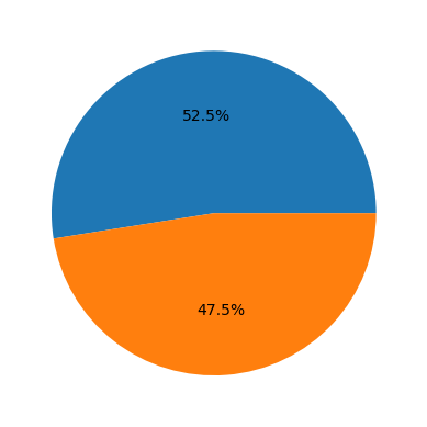
sizes = df['Productivity'].value_counts(sort=1)
plt.pie(sizes, autopct='%1.1f%%')
([<matplotlib.patches.Wedge at 0x206cc3afb80>,
<matplotlib.patches.Wedge at 0x206cc3b9310>],
[Text(-0.08630492316306847, 1.096609073570804, ''),
Text(0.08630482049111692, -1.0966090816512493, '')],
[Text(-0.04707541263440097, 0.598150403765893, '52.5%'),
Text(0.04707535663151831, -0.5981504081734086, '47.5%')])
- STEP2: DROP IRRLEVANT DATA 丢弃无关数据
python
df.drop(['Images_Analyzed'], axis=1, inplace=True)
df.drop(['User'], axis=1, inplace=True)
df.head()| Time | Coffee | Age | Productivity | |
|---|---|---|---|---|
| 0 | 8 | 0 | 23 | Good |
| 1 | 13 | 0 | 23 | Bad |
| 2 | 17 | 0 | 23 | Good |
| 3 | 22 | 0 | 23 | Bad |
| 4 | 8 | 2 | 23 | Good |
- STEP3: DEAL WITH MISSING VALUES 处理缺失数据
python
df = df.dropna()- STEP4: CONVERT NON-NUMERIC TO NUMERIC
将 Good 和 Bad 替换成计算机便于理解的数字类型
python
df.Productivity[df.Productivity == 'Good'] = 1
df.Productivity[df.Productivity == 'Bad'] = 2
df.head()| Time | Coffee | Age | Productivity | |
|---|---|---|---|---|
| 0 | 8 | 0 | 23 | 1 |
| 1 | 13 | 0 | 23 | 2 |
| 2 | 17 | 0 | 23 | 1 |
| 3 | 22 | 0 | 23 | 2 |
| 4 | 8 | 2 | 23 | 1 |
- STEP 5: PREPARE THE DATA(define indep/dep variables)
python
Y = df['Productivity'].values
Y = Y.astype('int')
Y
array([1, 2, 1, 2, 1, 2, 1, 1, 1, 2, 1, 1, 1, 2, 2, 2, 1, 2, 1, 2, 1, 2,
1, 2, 1, 2, 1, 2, 1, 2, 2, 2, 1, 2, 1, 2, 1, 2, 1, 2, 1, 2, 1, 1,
1, 2, 2, 2, 1, 2, 1, 2, 1, 2, 1, 2, 1, 2, 1, 2, 1, 2, 2, 2, 1, 2,
1, 2, 1, 2, 1, 2, 1, 2, 1, 2, 1, 2, 2, 2])
python
X = df.drop(labels=['Productivity'], axis=1)
X.head()| Time | Coffee | Age | |
|---|---|---|---|
| 0 | 8 | 0 | 23 |
| 1 | 13 | 0 | 23 |
| 2 | 17 | 0 | 23 |
| 3 | 22 | 0 | 23 |
| 4 | 8 | 2 | 23 |
- STEP 6: SPLIT DATA
python
from sklearn.model_selection import train_test_split

X_train, X_test, y_train, y_test = train_test_split(X, Y, test_size=0.1, random_state=20)
X_train.head()| Time | Coffee | Age | |
|---|---|---|---|
| 42 | 18 | 4 | 31 |
| 5 | 13 | 2 | 23 |
| 54 | 17 | 2 | 45 |
| 12 | 8 | 6 | 23 |
| 78 | 17 | 6 | 52 |
- STEP 7: DEFINE THE MODEL
python
from sklearn.linear_model import LogisticRegression

model = LogisticRegression()
model.fit(X_train, y_train)- STEP 8: TESTING THE MODEL
python
prediction_test = model.predict(X_test)
prediction_test
array([2, 2, 2, 1, 1, 2, 1, 2])
- STEP 9: VERIFY THE ACCURACY 验证准确性
python
from sklearn import metrics

print('Accuracy =', metrics.accuracy_score(y_test, prediction_test))
Accuracy = 0.75
- STEP 10: WEIGHTS
python
model.coef_array([[0.18788991, 0.19204588, 0.0200644 ]])
python
weights = pd.Series(model.coef_[0], index=X.columns.values)
weights
Time 0.187890
Coffee 0.192046
Age 0.020064
dtype: float64